Advanced Portfolio Construction and Analysis with Python - Recording Notes 01a
Course:
Advanced Portfolio Construction and Analysis with Python
Ref.: https://www.coursera.org/learn/advanced-portfolio-construction-python/
Jupyter NB Notebook ipynb - Labs and Codes: https://www.coursera.org/learn/advanced-portfolio-construction-python/ungradedLab/RqxtJ/labs-and-code/lab?path=%2Ftree

Module#1 - a) Introduction to Factor Investing
Q3: Some investors consider Oil Prices to be an important factor in determining equity returns. This would be an example of: (choose one)
- a) Macro Factor
- b) Style Factor
- c) Statistical Factor
- a) Macro Factor: Oil prices are likely to affect stock returns, but it is neither a statistical artifact nor is it intrinsic to the stock itself.
Module#1 - b) Factor Models and the CAPM
Q1: If a factor model is a good and accurate representation of what we see in the data, the epsilon term will be: (choose one)
- a) LOW
- b) HIGH
- Epsilon in the factor model refers to the error term, and is a measure of what might be in the data that is not captured by the factor model


CAPM, or the Capital Asset Pricing Model, is a financial model used to determine the expected return on an investment based on its risk relative to the market. It establishes a linear relationship between the expected return of an asset and its systematic risk, represented by beta (β).
Key Components of CAPM:
-
Expected Return (E(R)): The return an investor expects to earn from an investment.
-
Risk-Free Rate (Rf): The return on an investment with zero risk, typically represented by government bonds.
-
Beta (β): A measure of an asset's sensitivity to market movements. A beta of 1 indicates that the asset moves with the market, less than 1 indicates lower volatility, and greater than 1 indicates higher volatility.
-
Market Return (E(Rm)): The expected return of the market portfolio.
CAPM Formula:
The CAPM can be expressed with the following formula:
Where:
- = Expected return of the asset
- = Risk-free rate
- = Expected return of the market
- = Beta of the asset
Implications of CAPM:
- Risk and Return: CAPM demonstrates that higher risk (captured by beta) leads to higher expected returns.
- Investment Decisions: Investors can use CAPM to evaluate whether the return of an asset justifies its risk, aiding in portfolio construction and capital allocation.
Limitations:
- Assumes a linear relationship between risk and return.
- Relies on historical data to estimate beta, which may not predict future performance.
- Assumes markets are efficient and that all investors have the same information.
Overall, CAPM is a foundational concept in finance that helps in understanding the trade-off between risk and return in investment decisions.
===== ===== =====Q2:What is CAPM? According to the CAPM, the alpha term in the CAPM Factor Model is:
- a) Zero
- b) One
- c) Zero if Epsilon is Zero, One otherwise
- d) Depends on the Risk Free Rate
- ans.: a) -- In the Capital Asset Pricing Model (CAPM), the alpha (α) represents the excess return of an investment relative to the return predicted by its beta (β) and the market risk premium. The CAPM assumes markets are efficient, meaning all assets are fairly priced, and no investor can consistently achieve abnormal returns. Under this assumption:
- α = 0 (theoretical expectation), as the asset’s return is fully explained by its systematic risk (beta) and the market return.
- A non-zero alpha in practice indicates outperformance (α > 0) or underperformance (α < 0) relative to the CAPM prediction.
- Why Other Options Are Incorrect:
- b) One: Alpha is not a fixed coefficient; it measures deviation from expected returns.
- c) Zero if Epsilon is Zero: Epsilon (ε) represents idiosyncratic risk, but alpha is zero regardless of ε under CAPM.
- d) Risk-Free Rate Dependency: Alpha is independent of the risk-free rate; it reflects performance relative to the CAPM equation.
CAPM Formula:
by definition in an efficient market.
Here,
Module#1 - c) Multi-Factor models and Fama-French

Size effect: (value stock outperforms growth stock)

Q1: A Manager tells you that he concentrates his portfolio in Value stocks because Value outperforms Growth, and his portfolio has outperformed the S&P500 for the last 3 years. Assuming his statements are all True, which of the following statements can you conclude from this information. (which one?)
- a) The portfolio will outperform the S&P500 next year
- b) The portfolio will outperform the S&P500 next year if the Value factor has a positive risk premium next year
- c) If the manager does not show style drift AND the Value Factor generates a positive risk premium the next year, THEN the manager is likely to outperform, but it is not a certainty
- d) None of the Above
- ans. c) This statement acknowledges the conditions under which the manager's strategy could continue to be successful while recognizing that past performance does not guarantee future results. The Factors Mimicking Portfolios are broad portfolio and it is possible to see a return that is different from the Factor Mimicking portfolio
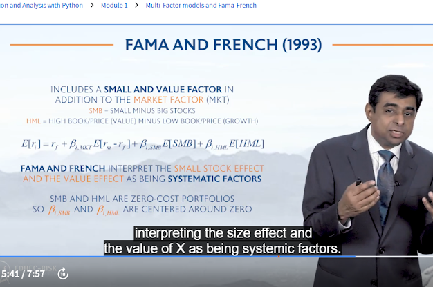

Q1. The Original Fama French Factor (1993) Model is: (which one?)
- a) a TWO factor model where the factors are Value and Size
- b) a THREE factor model where the factors are Market, Value and Size
- c) a FOUR factor model where the factors are Market, Value, Size and Momentum
- d) a FIVE factor model where the Factors are Value, Growth, Small Cap, Large Cap and Market
- b) ans. The Fama French model extends the CAPM by adding Value and Size as Factors
Module#1 - d) Factor benchmarks and Style analysis

Q1) Assume the risk free rate is 1% per year and the Stock Market returned 11% in a given year. An Active Manager “beat the market” and generated a 14% return and had a Beta of 1.3: (which one?)
- a) The Manager generated Zero Alpha
- b) The Manager generated Positive Alpha
- c) The Manager generated Negative Alpha
- ans a). Since the excess return of the manager (14% - 1% = 13%) is exactly equal to the beta times the excess return of the market (1.3x(11-1)), the alpha is zero
- CAPM model to determine the manager's alpha: Expected Return =Risk-Free Rate+β×(Market Return−Risk-Free Rate),
- where Risk-Free Rate = 1%, Market Return = 11%, Manager's Return = 14% and Beta = 1.3 ==> Expected Return=1%+1.3 × (11% − 1%) = 1% + 1.3×10% = 1% +13% = 14% ==> Now, we can find the alpha: Alpha = Actual Return − Expected Return = 14%−14% = 0%

Model & Quality of Fit:

Manage value add = alpha
Q2: For Sharpe Style Analysis, the coefficients that we compute are constrained to sum to 1. This is done so that: (which one?)
- a) They can be interpreted as portfolio weights in the explanatory indices
- b) To impose a Long-Only constraint
- c) To speed up the calculation
- d) To make sliding window analysis easier
- ans. a): The coefficients are interpretable as weights if they sum to 1 and are all positive.


Q3: Sharpe Style Analysis can be used to measure Style Drift
- a) TRUE
- b) FALSE
- ans. is True: a Sliding window analysis over time can reveal style drift in a manager.
Module#2 - a) Shortcomings of cap-weighted indices
- Default approach is to use a cap-weighted (CW) index as a benchmark for active or passive managers.


Module#2 - b) From cap-weighted (CW) benchmarks to smart-weighted benchmarks
- Shortcoming #1: CW Indices provide an inefficient diversification of unrewarded and specific risks.
- Solution: Use a smarter weighting scheme.
- Shortcoming #2: CW Indices provide an inefficient exposure to rewarded systematic risks.
- Factors: a) size, b) book-to-market.
- Solution: ???


Step #2) Select your preferred weighting scheme.

Smart Factor Benchmarks are better rewarded.


Suppose the estimation of a GARCH(1,1) model on daily data gives:

and also suppose the last daily estimate of the volatility is 1.6% per day and the most recent percentage change in the market variable is 1%. What is the new daily volatility estimate?
- The answer is 1.53%. The new variance estimate is: 0.000002 + 0.13 x 0.0001 + 0.86 x 0.000256 = 0.00023516. Taking the square root, we obtain the new volatility estimate as 1.53% per day.


留言
張貼留言